In demand planning, Forecast accuracy assesses how closely a forecast matches actual demand. It is often used as a performance indicator, similar to service level or inventory level.
In many organizations, including at Pawa, forecast accuracy is often expressed through an aggregated score, derived from a relative error and used as a high-level indicator.
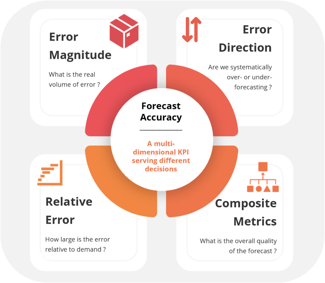
In this article, we adopt a broader approach, considering forecast accuracy as a set of complementary measures, necessary to analyze and resolve operational issues.
These measures do not share the same objective, scope, or relevance depending on the decisions they support.
Demand forecasts support very different decisions. They serve first and foremost to support demand and production.
Thus, depending on requirements, they can be used to size production capacities, allocate budgets, manage inventories, secure an industrial plan, or align sales and operations teams.
These decisions are not based on the same time horizons, do not expose the company to the same risks, and do not tolerate the same types of errors. In this context, no single metric can satisfactorily address all of these challenges. An aggregated measure may indicate that the forecasts are generally consistent with the business trajectory, while a more detailed one will highlight significant discrepancies for certain products, periods, or geographical areas. These view are not complementary : they reflect different analytical needs.
Attempting to manage all decisions based on a single accuracy measure often leads to rough trade‑offs and a partial understanding of operational reality.
Forecast accuracy measures can be grouped into a few broad categories, all serving different business needs.
The table below provides an overview of the main forecast accuracy measures and how they support different business decisions. The remainder of the article examines each of these categories of measures in more detail, in order to clarify their benefits and limitations.
Type of decision | What we seek to understand | Type of relevant metric | Main roles concerned |
Capacity planning | Actual magnitude of the volume gap | Absolute error (MAE) | Demand planner, production planner, production teams |
Inventory management | Risk of overstock or stockout | MAE (%) + bias (%) | Supply chain, finance |
Portfolio review | Comparability between products, markets or channels | MAE (%) | Demand planning team, management, commercial operations |
Forecast governance | Systematic forecasting stance (over- or under-forecasting) | Bias (%) | Head of demand planning, management |
S&OP arbitration | Overall impact and nature of business risk | Pawa Score | S&OP team, operations management, finance |
What follows adopts an approach that is primarily conceptual and business-oriented: the objective is to clarify what each type of measure seeks to qualify, rather than dwelling on the calculations.
In practice, these measures rely on the ability to compare the observed demand with forecasts formulated at different points in the past. Pawa precisely makes it possible to go back in time, to visualize the forecasts as they existed at a given moment, and to analyze the accuracy of the forecasts based on these past forecasts.
For details of the mathematical formulas as well as the principles for configuring these indicators, particularly with regard to the choice of the measurement horizon, which may vary significantly depending on needs and teams, you may refer to the article dedicated to their operational implementation (article 3).
Absolute error measures aim to quantify the average deviation between the forecast and the observed demand, expressed in the same units as the demand (units, pallets, MWh, etc.).
As such, they describe the magnitude of the errors in actual volume and answer a simple question: by how much does the forecast deviate, on average, from reality?
These measures enable, for example, a logistics team to translate a forecast deviation into concrete impacts: storage capacity, picking workload, risk of stockout or overstock.
Let us consider a very concrete situation. A factory must prepare the production of a monthly batch of a food product packaged in sachets. The forecast estimates demand at 1,000 boxes, while the actual observed demand ultimately reaches 1,150 boxes. Thus, the absolute deviation for the period is 150 boxes. Over several months, an MAE of 150 means that, on average, planning is off by 150 boxes per production cycle. For operational teams, this is not a theoretical value : it corresponds to an additional half-pallet rack to store, an unplanned hour of production, or an additional delivery round. The MAE thus makes it possible to reason directly in operationally meaningful volumes, real costs, capacity, and operational workload.
Nonetheless, since these measures do not relate the error to the level of activity, their interpretation becomes more difficult when products, markets, or channels of very different sizes are compared: the same absolute deviation may represent a major error in a small scope and a negligible deviation in a large one. If product A sells 1,000 units per month and product B 10,000 units per month, an identical MAE of 150 units does not carry the same significance : it represents around 15% of the volume for A, but only 1.5% for B.
Put differently, absolute measures describe the actual size of the error well, but not its relative importance, hence the value of complementing them with indicators expressed as a percentage when comparing heterogeneous scopes.
In summary | |
What the measure indicates | The actual magnitude of the error in volume (units, pallets, MWh, etc.) |
What it does not indicate | The relative significance of the error in relation to the level of activity |
To whom it is addressed | Demand planners, production, logistics |
Risk if used alone | Poor comparability between products or scopes of different sizes |
Bias measures seek to identify in which direction forecasts deviate from reality. They highlight the existence of a systematic tendency to over-forecast or under-forecast by observing whether, on average, errors are rather positive or negative.
Hence, they answer a different question from that of absolute error measures: not “by how much does the forecast deviate from reality?”, but “in what direction is the error repeated over time?” In other words, they shed more light on the forecasting behaviour than on its level of accuracy.
These measures are of particular interest in environments where forecasts are largely influenced by human adjustments or by implicit management rules. A persistent bias may, for example, reveal a systematic tendency to over-protect inventory, to overestimate demand in order to safeguard capacity, or to systematically under-forecast in contexts of production constraints or conservative commercial objectives.
Let us suppose we are part of a cosmetics company in which sales teams regularly adjust forecasts upwards before production, for fear of stockouts during promotional peaks. Over six consecutive months, actual demand is systematically below forecasts: +90 units, +120 units, +85 units, +110 units, +95 units, +130 units. On average, the error remains positive: the bias measure clearly highlights a structural tendency towards over-forecasting.
On the finance side, bias sheds light on more global indicators such as the immobilisation of cash, rising storage costs, but also the increase in the rate of expired or devalued products at the end of the cycle, which is particularly critical for ranges with a limited shelf life. Simply put, the bias measure here becomes a behavioural and economic diagnostic tool, revealing a tendency to over-protect.
In contrast, bias measures have a major limitation: since they retain the sign of the errors, positive and negative deviations can offset each other. A series of large over-forecasts followed by large under-forecasts may thus lead to an average bias close to zero, even though the forecast is highly unstable and unreliable. This is why the absence of bias does not imply good accuracy, but only an average balance between excess and deficit in forecasting.
This limitation becomes clear when illustrated through a concrete case.
Let us suppose that a product displays the following deviations over four months between forecast and actual demand: +120 units, +140 units, −130 units and −150 units. The average of these errors is close to zero, which suggests zero bias. However, each month shows significant deviations, and the forecast remains highly erratic. In this case, the bias measure masks the volatility of the errors and should be complemented with a measure of absolute error.
This means that bias measures are essential for understanding the structural orientation of forecasts, but they do not provide information on the actual magnitude of deviations. They must be read in conjunction with error measures, and not as a standalone indicator of forecast quality.
| In summary |
What the measure indicates | The direction in which the forecast systematically deviates from reality (over- or under-forecasting) |
What it does not indicate | The actual magnitude of the deviations in volume |
Whom it addresses | Planning managers, management, finance |
Risk if used alone | Masking of significant errors through offsetting positive and negative deviations |
Percentage-based accuracy measures seek to provide a relative understanding of the error, independently of the volume level. They answer a different question than absolute error metric: how large is the error relative to demand?
This approach offers a major advantage when it comes to comparing heterogeneous scopes: products, markets, countries or channels whose activity levels are very different. An error of 150 units does not have the same meaning when selling 1,000 or 10,000 units; expressed as a percentage, however, it becomes comparable across contexts. This is what makes MAE% a particularly useful indicator for cross-functional monitoring, portfolio management or communication with non-technical teams.
This benefit becomes clear in a common operational situation. A management team seeks to compare the forecasting performance of two product families: high-volume strategic products and long-tail products. By expressing the error as a percentage, the manager can identify that certain long-tail items show an average deviation of 25%, compared with 6% for core-range products, information that cannot be derived from errors expressed solely in units. Here, the percentage-based measure serves its purpose : it makes it possible to dectec priorities at portfolio level.
However, this normalization also has its limits. In low-volume contexts, a small variation in units can lead to very high percentages, which give an exaggerated picture of the error. On the other hand, an apparently satisfactory percentage may conceal large deviations in absolute volume and a significant operational impact. Put differently, these measures facilitate comparison, but they can dilute the materiality of the deviations if used in isolation.
This ambiguity becomes clear when illustrated with a concrete case. Suppose a product sells an average of 10,000 units per month. An error of 200 units corresponds to a 2% deviation, which may seem acceptable from an overall perspective. However, these 200 units may represent several additional pallets to be stored, an increase in logistics costs, or a stockout at a key point of sale: their impact remains very real, even if the percentage appears low.
Conversely, another product sells an average of 50 units per month. An error of 10 units here corresponds to a 20% deviation, which gives the impression of a very poor forecast, whereas in reality the operational impact remains limited. The percentage correctly reflects the proportion of the error, but not necessarily its economic severity.
In summary, percentage-based accuracy measures are excellent indicators for comparability and overall management, but they do not replace measures expressed in actual volume. Their interpretation becomes more relevant when they are considered alongside absolute errors and the business context, in order to reconcile statistical comparability with operational relevance.
| In summary |
What the measure indicates | The size of the relative error in relation to the demand |
What it does not indicate | The actual operational impact in volume |
Who it targets | Management, planning, portfolio management |
Risk if used alone | Over-interpretation of errors on low volumes or underestimation of impacts on high volumes |
Composite scores and measures seek to go beyond a one-dimensional perspective on forecast performance by combining several dimensions of error within a single indicator. Whereas an isolated measure describes either the magnitude of deviations or their direction, a composite score aims to provide a more holistic and pragmatic view of forecast quality, by integrating for example both the size of the error and the possible presence of a structural bias.
From this perspective, some organizations opt for simple yet robust approaches, consisting of tracking two complementary indicators simultaneously rather than a single score. This is notably the case in Pawa, where forecast performance is assessed through a combination of MAE (mean absolute error) and bias measures. The MAE makes it possible to assess the concrete magnitude of deviations in volume, while the bias provides information on the systematic direction of the forecast (consitently above or below demand). Together, these two readings offer a richer diagnosis than each taken in isolation.

This can be illustrated with a concrete situation. Two product families show an identical MAE of 180 units. If we look only at this measure, they appear to present the same level of risk for operations. But the bias analysis reveals two very different realities: in the first family, the errors are almost always positive, indicating a structural over-forecast that leads to high inventory levels, write-downs and, from a finance perspective, an increase in the rate of obsolete products. In the second family, the bias is close to zero but the errors alternate between over- and under-forecast, mainly generating operational volatility (workload variability, frequent readjustments, occasional capacity constraints).
In this case, the combination of MAE and bias makes it possible to distinguish between two types of problems that do not call for the same actions: on the one hand, an issue of attitude and governance of forecasting; on the other, an issue of process stability and signal quality. It is precisely this type of enriched interpretation that composite measures make possible.
Other approaches go further by integrating business-specific weightings or economic dimensions: value-driven prioritization, product criticality, cost of stockout or overstock, or indicators such as the actual added value of the forecast (FVA —> Forecast Value Added) aimed at measuring the real contribution of human adjustments compared with a statistical baseline. These scores can be particularly useful in complex environments, where the question is not only to measure the error, but to understand where it really matters and how it translates into operational impact.
However, they present an important limitation: the more dimensions a score integrates, the more it risks becoming opaque. When the construction logic is not explicitly documented (choice of weightings, role of each component, calculation conventions), the score can be difficult to interpret and may even lead to biased decisions.
In practice, composite measures can offer a richer view that is closer to the real challenges, provided that their design remains transparent, explainable, and aligned with business objectives.
| Summary |
What the measure says | An enhanced understanding combining several dimensions of the error |
What it does not say | The exact contribution of each component if the score is not well explained |
To whom it speaks | S&OP, operations management, finance |
Risk if used alone | Lack of interpretability if the construction of the score is not transparent |

No single measure can, on its own, account for the complexity of supply chain challenges. Each indicator provides a partial, sometimes biased view of reality. It is precisely for this reason that their combination, their contextualization, and their business-focused interpretation are crucial.
As a result, organizations are faced with the challenge of constructing a view of forecasting performance that is suited to the decisions to be supported, the risks to be managed, and the behaviors to be understood. When used in a complementary and contextualized manner, accuracy measures then become valuable tools for decision support.
Which forecast accuracy measures are available in Pawa?
This article presents the main forecast accuracy measures available in Pawa and provides a short interpretation for each of them.
How to configure a forecast accuracy measure in Pawa
This article explains how to configure sales forecast accuracy in Pawa.